Exploring Stock Data with a Yahoo Finance Python Module

A beginner’s guide for retail investors enthused by studying stocks

If you are a retail investor who is interested in the stock market, it is essential to research the stocks on your own. Yahoo Finance, among many other websites, provides stock data for users to interact with. For those who are versed with coding skills, there are a few API’s (application program interface) for programmatic access to Yahoo Finance data. yfinance, maintained by Ran Aroussi, is a Python module that provides access to multiple datasets.

This post will demonstrate some aspects of the yfinance module, and hopefully open the gateways for others to engage and explore.

Installation

I used pip to install. In Terminal, run the following:

pip install yfinance

Ticker Module

To access data for a single stock, simply use the Ticker module. First, import yfinance, then initiate by defining the ticker symbol you are interested in (e.g., Amazon, by sybmol AMZN).

import yfinance as yf
stock = yf.Ticker('AMZN')

The stock instance contains tons of information, which you can access by calling different methods. We will walk through them in the following sections, but first let us look at the info object by printing out stock.info. This contains, in a dictionary, basic information about the Amazon business and the AMZN stock, including price, volume, short interest, and exposure to beta factor.

{'zip': '98109-5210',
 'sector': 'Consumer Cyclical',
 'fullTimeEmployees': 1298000,
 'longBusinessSummary': 'Amazon.com, Inc. engages in the retail sale of consumer products and subscriptions in North America and internationally. The company operates through three segments...,
 'city': 'Seattle',
 'phone': '206-266-1000',
 'state': 'WA',
 'country': 'United States',
 'companyOfficers': [],
 'website': 'http://www.amazon.com',
 'maxAge': 1,
 'address1': '410 Terry Avenue North',
 'industry': 'Internet Retail',
 'previousClose': 3146.14,
 'regularMarketOpen': 3143.47,
 'twoHundredDayAverage': 3209.0454,
 'trailingAnnualDividendYield': None,
 'payoutRatio': 0,
 'volume24Hr': None,
 'regularMarketDayHigh': 3163.52,
 'navPrice': None,
 'averageDailyVolume10Day': 3790100,
 'totalAssets': None,
 'regularMarketPreviousClose': 3146.14,
 'fiftyDayAverage': 3237.417,
 'trailingAnnualDividendRate': None,
 'open': 3143.47,
 'toCurrency': None,
 'averageVolume10days': 3790100,
 'expireDate': None,
 'yield': None,
 'algorithm': None,
 'dividendRate': None,
 'exDividendDate': None,
 'beta': 1.143009,
 'circulatingSupply': None,
 'startDate': None,
 'regularMarketDayLow': 3087.12,
 'priceHint': 2,
 'currency': 'USD',
 'trailingPE': 73.97872,
 'regularMarketVolume': 2506444,
 'lastMarket': None,
 'maxSupply': None,
 'openInterest': None,
 'marketCap': 1558297051136,
 'volumeAllCurrencies': None,
 'strikePrice': None,
 'averageVolume': 3656136,
 'priceToSalesTrailing12Months': 4.03637,
 ...
 'shortPercentOfFloat': 0.0089,
 'sharesShortPriorMonth': 3141707,
 'impliedSharesOutstanding': None,
 'category': None,
 'fiveYearAverageReturn': None,
 'regularMarketPrice': 3143.47,
 'logo_url': 'https://logo.clearbit.com/amazon.com'}

Price History

The history method provides access to the price history of a certain stock. Below are the input arguments for calling the method, from the module’s documentation.

history(period='1mo', interval='1d', start=None, end=None, prepost=False, actions=True, auto_adjust=True, back_adjust=False, proxy=None, rounding=False, tz=None, **kwargs)

Let’s use the default period of 1 month to obtain the data, and inspect.

prices = stock.history(period='1mo')
prices.head()

And this shows us the first 5 rows of the dataframe

First 5 rows of the price history

In order to calculate the daily returns of the stock, we can use the pct_change method of pandas on the Close column as follows

prices['Returns'] = prices['Close'].pct_change()
prices.head()

Now the dataframe has a returns column which can be used for different purposes, e.g. calculating rolling returns over certain time periods.

First 5 rows of the price history with a Returns column

In addition, the history method provides real time price data. For those who are interested, this can be used to monitor and even trade stocks intra-day. To show how the data is real time, we access 1 day data, pause for 1 minute, and access 1 day data again. The price data would be in the Close column. Code below

print(datetime.now())
display(stock.history(period='1d'))
time.sleep(60)
print(datetime.now())
display(stock.history(period='1d'))

Data printed out as follows

Real time data of Amazon (AMZN)

Dividend History

For investors who are interested in dividend investing, the dividends method provides historical dividend payout data. An example is shown below for the past 8 quarters of dividends from Visa. One could merge this with price history to calculate dividend yield, compare different yields and pick high yield investments.

stock = yf.Ticker('V')
stock.dividends.tail(8)

Visa (V) dividend history for the past 8 quarters

Major Shareholders

For investors who are interested in the ownership of stocks, two objects under Ticker can provide ownership data. This could be useful to devise strategies to follow insightful large investors in what they invest, and capture some returns.

Below, we show Palantir’s largest investors (Holder column) and how much of outstanding shares they own of Palantir (Shares and % Out columns). You can also find out when the holding was last reported (Date Reported column), which, I believe, is the date when the firm filed its SEC 13F form.

stock = yf.Ticker('PLTR')
stock.institutional_holders

Institutional holders of Palantir (PLTR)

stock.mutualfund_holders

Mutual fund holders of Palantir

Analyst Recommendations

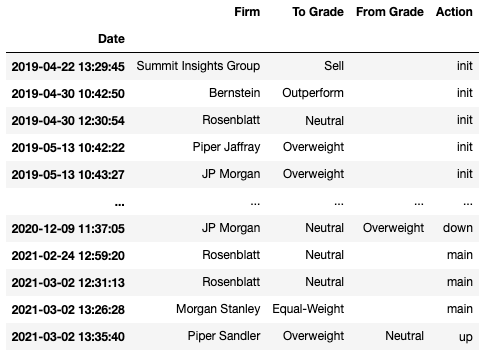
Wall Street analysts provide their recommendations on stocks, which are sometimes Buy, Hold, and Sell, from bullish to bearish; or it could be Overweight (OW), Equal-Weight (EW), and Under-Weight (UW). This can be useful to inspect if there is a consensus on a stock, and monitor actions of upgrading or downgrading a stock, which at times can affect share prices.

stock = yf.Ticker('ZM')
stock.recommendations

In the dataframe below, we find when the recommendation was published, in the Date index; the firm, or broker, the analyst is affiliated with; the recommendations and the prior recommendations, in “To Grade” and “From Grade” columns; and the “Action”, i.e. the delta between From and To, which could be

• Init: initiation
• Down, or Up: downgrade or upgrade
• Main: maintain previous recommendation

Analyst recommendations for Zoom (ZM)

Calendar

For investors on the lookout of certain stocks’ upcoming earnings, the calender method provides information on the date of the next earning and what the Wall Street estimates are. In the example below, we find Tesla’s upcoming earnings date. Since the date is not confirmed yet, the dataframe contains two columns for two estimated dates. It contains the average, minimum and maximum of Earnings per Share (EPS) and Revenue, two important valuation metrics.

stock = yf.Ticker('TSLA')
stock.calendar

Tesla (TSLA) upcoming earnings date and estimates

Options

Last but not least, the Ticker module provides data on option pricing data for those interested. You can first use the options object to find the expiry dates, stored in a tuple.

stock = yf.Ticker('AMZN')
stock.options

AMZN options expiry dates

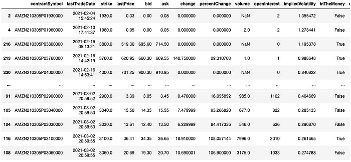
Then, use the option_chain method to access option data, by defining the expiry date. Then, access calls and puts separately as follows. You would find the trade date, strike price, bit & ask price for the contract, trading volume, implied volatility (IV), among other information.

option_chain = stock.option_chain(date='2021-03-05')
option_chain.calls.sort_values('lastTradeDate')

Call option history for AMZN

option_chain.puts.sort_values('lastTradeDate')

Put option history for AMZN

Conclusion

Hope this is useful for those who are interested in applying coding to stock research and investing. Good luck to all!